Time Variance

Contents

1. Intro to SPICE Algorithm
2. Framework and your first circuit!
3. More Static Linear Components
4. Nonlinear and Diode
5. MOSFET
6. Time Variance (this article)
7. Applications

Now let’s add another dimension to our simulation: time

Framework

We will use Euler’s method to make a linear approximation of time varying components with memory (cap, ind) with respect to time. This is very similar to Newton’s method, but with time as the x-axis. The component will be modelled by a current source parallel to a resistor.

This will be the outer loop of the SPICE algorithm:

1. stamp() the component to get its linear model
2. solve() an operating point
3. update() the memory
4. Advance a time step

Time Varying Sources

This part is designed and written by Andrew Yang and Faustina Cheng :)

Time varying sources do not have memory. We just need \(t\) as a parameter to get its value at \(t\).

We’ll design new signatures for independent sources. We’ll show how AC functions are implemented. Again, declare a wrapper around the union on each parameter type.

typedef struct {
    double vo;
    double va;
    double fo;
    double td;
    double a;
    double phase;
} SpiceSinParams;

typedef struct {
    double dc_value;
} SpiceDCParams

typedef enum {
    SPICE_FUNC_SIN,
    SPICE_FUNC_DC
} SpiceFuncType;

typedef struct {
    SpiceFuncType type;
    union {
        SpiceSinParams sin;
        SpiceDCParams dc;
    } params;
} TransientSource;

The stamping function needs to be updated

void isrc_stamp(Component *c, float Gm[][MAT_SIZE], float I[]) {
    (void)Gm;
    ISrc *s = &c->u.isrc;
    TransientSource *src = s->src;
    float Ieq;
    if (src->type == SPICE_FUNC_SIN) {
        SpiceSinParams *params = &src->params.sin;
        Ieq = params->vo + params->va * exp(-params->a * (t - params->td)) * sinf(2.0f * M_PI * params->fo * (t - params->td) + params->phase / 360.0f);
    } else if (src->type == SPICE_FUNC_DC) {
        Ieq = src->params.dc.dc_value;
    } else {
        printf("vsrc_stamp: unknown source type\n");
        exit(1);
    }

    int n1 = s->n1, n2 = s->n2;
    if (n1 != -1) I[n1] += Ieq;
    if (n2 != -1) I[n2] -= Ieq;
}

As an exercise, implement the SPICE pulse source

State Holding Elements

Now to the real challenge: stamping and updating capacitors.

We used the Backwards Euler’s method: compute \(\frac{dv}{dt}\) of the next time step, and use it as the slope of the current approximation. A future work would be to use a better approximation method, such as trapezoidal or Runge-Katta

Definition

typedef struct { 
    int n1, n2;             // nodes
    float C, dt;            // device constants
    float v_prev;           // previous values
} Cap;

Registration

void add_cap(int n1,int n2,float C,float dt,float v0) {
    Component *c = &comps[ncomps++];
    c->type      = LIN_T;
    c->stamp_lin = cap_stamp_lin;
    c->stamp_nl  = NULL;
    c->update    = cap_update;
    c->u.cap     = (Cap){n1,n2,C,dt,v0};   // initial conditions are 0
}

Stamping

I might be off by 1

void cap_stamp_lin(Component *c, float Gm[][MAT_SIZE], float I[]) {
    Cap *p = &c->u.cap;
    float Gc  = p->C / p->dt;
    float Ieq = -Gc * p->v_prev;

    int n1 = p->n1, n2 = p->n2;
    if (n1 != -1) Gm[n1][n1] += Gc;
    if (n2 != -1) Gm[n2][n2] += Gc;
    if (n1 != -1 && n2 != -1) {
        Gm[n1][n2] -= Gc;
        Gm[n2][n1] -= Gc;
    }
    if (n1 != -1) I[n1] -= Ieq; // Ieq is defined leaving n1, entering n2
    if (n2 != -1) I[n2] += Ieq;
}

Updating

void cap_update(Component *c) {
    Cap *p = &c->u.cap;
    float vc = (p->n1!=-1? v[p->n1]:0) - (p->n2!=-1? v[p->n2]:0);
    float Gc = p->C / p->dt;
    float Ieq = -Gc * vc;

    p->v_prev = vc;
}

Inductors are exactly the same, if not easier, since there is no need to convert to a Norton current source

Simulation Loop

This simulation will be an outer loop around the operating point Newton loop.

• CircuitCim keeps a local copy of the static and outer loop results, so it doesn’t have to re-stamp every component. Some memcpy()s need to be updated to reflect that

  /* Main loop: linear and nonlinear */
  for (int n = 0; n < nsteps; n++) {
    t = n * time_step;
    // 0. retrieve static component matrix
    clear_system_sta();
  
    // 1. stamp all linear components
    for (int i = 0; i < ncomps; i++) {
        if (comps[i].type == LIN_T && comps[i].stamp) {
            comps[i].stamp(&comps[i], G, Ivec);
        }
    }
  
    // 2. Snapshot G, I with only linear components, and previous v
    float prev_v[MAT_SIZE];
    memcpy(G_lin, G, sizeof G);
    memcpy(I_lin, Ivec, sizeof Ivec);
    memcpy(v_prev, v, sizeof v);
  
    // 3. Newton-Raphson loop for all nonlinear components
    operaing_point()    // defined before
  
    // 4) final update so device states match the converged voltages
    for (int i = 0; i < ncomps; i++) {
        if (comps[i].type == LIN_T && comps[i].update) {
            comps[i].update(&comps[i]);
        }
    }
  }
  

LRC Circuit

With this, we can test out a second-order LRC circuit:

float time_step = 5e-6f;
int nsteps = 2000;

void setup(void) {
    add_vsrc(0, -1, 2, step5);
    add_res(0, 1, 10.0f);
    add_ind(1, 3,  1e-3f, time_step);
    add_cap(3, -1, 1e-6f, time_step);
    nnodes = 4;
}

Note that time step should be at least 10 times smaller than the smallest capacitor/inductor value for an accurate simulation.

Otherwise, it looks PERFECT!

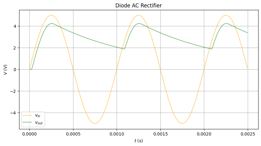
Rectifier

To test out both loops, let’s build a rectifier with a diode and a capacitor

float time_step = 5e-7f;
int nsteps = 500;

void setup(void) {
    add_vsrc(0, -1, 1, sin5);
    add_res(0, 2, 1.0f);
    add_diode(2, 3, 1e-15f, 0.025875f);
    add_cap(3, -1, 1e-6f, 5e-6f);
    nnodes = 4;
}

It simulates the iconic rectifier curve, with:

• Precise diode drop
• Exponential discharge (starts very linear)

Exercise: build a bridge rectifier.