Work in progress. More details to come!
Code and full results: mg-04/yolov8-project

A PyTorch fault-injection framework for YOLOv8n, used to find which weights and layers need protection in a secure-FPGA + Jetson deployment. It flips single bits in FP32 weights (memory faults) and activations (buffer and compute faults), then separates silent corruption from detectable corruption.

Method

• Target: YOLOv8n after BatchNorm fusion, 64 conv layers, ~3.1M parameters, evaluated on COCO
• Fault sites: weights, persistent activation faults, and transient (single-inference) activation faults
• Campaign: 64 layers × 16 targets × 6 bit positions × 3 sites = 18,432 injections
• Outcomes per image:
  • DUE: NaN/Inf in the output, detectable at runtime
  • SDC: clean-looking output with lost, phantom, or misclassified objects, not detectable
  • Benign / masked: detections unchanged or only slightly shifted

Key Findings

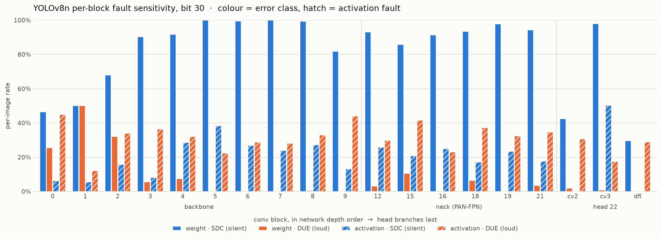
• One bit carries the risk. Bit 30, the FP32 exponent MSB, accounts for ~93% of random-fault risk. Flipping it scales a typical weight by \(2^{128}\)
• Weight faults are silent; activation faults are loud. At bit 30, weight faults are 83% SDC and 6% DUE, while activation faults are 23% SDC and 31% DUE
• Every other bit is undetectable. NaN/Inf appears only at bit 30, so faults at other bits never show up in the output
• The classification head is the most sensitive part of the network under every fault type

Detect Head

Three scales, two branches. Numbers are the per-image SDC rate under a bit-30 fault: W = weight fault, A = persistent activation fault. Red = most sensitive, green = least.

flowchart LR
    classDef hi fill:#c0392b,stroke:#7b241c,color:#fff
    classDef mid fill:#d68910,stroke:#9c640c,color:#fff
    classDef lo fill:#1e8449,stroke:#145a32,color:#fff
    classDef io fill:#5d6d7e,stroke:#34495e,color:#fff,stroke-dasharray:3 3
    P3(["P3 s8<br/>block 15"]) --> CV3
    P4(["P4 s16<br/>block 18"]) --> CV3
    P5(["P5 s32<br/>block 21"]) --> CV3
    P3 --> CV2
    P4 --> CV2
    P5 --> CV2
    CV3["cv3 · class branch<br/>W 98 · A 50<br/>MOST SENSITIVE"] --> OUT["out<br/>84 x 8400"]
    CV2["cv2 · box branch<br/>W 42 · A 0"] --> DFL["dfl · 16 params<br/>W 30 · A 0"] --> OUT
    class CV3 hi
    class CV2,DFL lo
    class P3,P4,P5,OUT io

The class branch (cv3) and the box branch (cv2) see the same inputs at the same depth, yet have opposite sensitivity. A corrupted class score poisons the NMS ranking for the whole image, while a corrupted box coordinate only misplaces one detection.